To get the data needed to render a chart, Charts creates a MongoDB Aggregation Pipeline and runs the pipeline on the MongoDB database server. The pipeline consists of multiple stages, each of which is generated based on different settings specified by the chart's author.
This document explains how the various Chart Builder settings are used to construct the Aggregation Pipeline. You can view the pipeline used to create a chart by choosing the View Aggregation Pipeline option in the Chart Builder's ellipsis dropdown on the top right.
Atlas Charts construct a pipeline that consists of the following segments in the following order:
Note
When creating a chart, you can configure some but not all of the previous chart segments. When Charts generates the aggregation pipeline, it skips unspecified segments.
Example
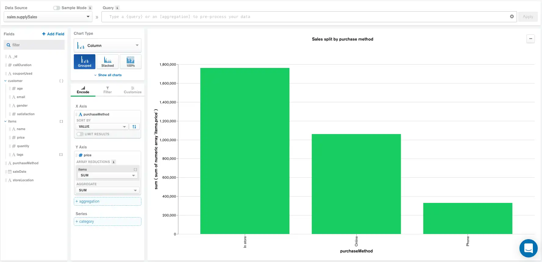
The following chart shows the total sale amounts from an office supply company, categorized by purchase method. Each document in the data collection represents a single sale.
Using this chart as an example, we will explore how the specifications for each of the above settings change the aggregation pipeline generated by Atlas Charts.

Encoding
Without any Data Source pipeline, Query bar queries, calculated fields, and filters added in the Filter pane, Atlas Charts generates the following aggregation pipeline:
1 { 2 "$addFields": { // Encoding 3 "__alias_0": { 4 "$sum": "$items.price" 5 } 6 } 7 }, 8 { 9 "$group": { 10 "_id": { 11 "__alias_1": "$purchaseMethod" 12 }, 13 "__alias_0": { 14 "$sum": "$__alias_0" 15 } 16 } 17 }, 18 { 19 "$project": { 20 "_id": 0, 21 "__alias_1": "$_id.__alias_1", 22 "__alias_0": 1 23 } 24 }, 25 { 26 "$project": { 27 "x": "$__alias_1", 28 "y": "$__alias_0", 29 "_id": 0 30 } 31 }, 32 33 { 34 "$addFields": { // Sorting 35 "__agg_sum": { 36 "$sum": [ 37 "$y" 38 ] 39 } 40 } 41 }, 42 { 43 "$sort": { 44 "__agg_sum": -1 45 } 46 }, 47 { 48 "$project": { 49 "__agg_sum": 0 50 } 51 }, 52 { 53 "$limit": 5000 54 }
The pipeline at this point consists of groups from the Encode panel, stages for the default sort order, and the maximum document limit, which is set to 5000 by Atlas Charts.
Adding Queries
The query below restricts the documents shown to only those with
a saleDate equal to or more recent than January 1, 2017 with at
least 5 elements in the items array. items is
an array where each element is an item purchased during a sale.
Query:
{ $and: [ { saleDate: { $gte: new Date("2017-01-01") } }, { 'items.4': { $exists: true } } ] }
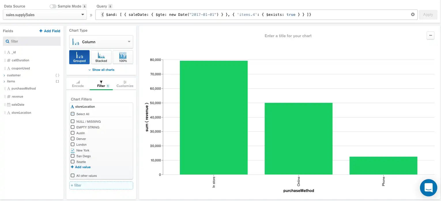
Applying the above query in the Query bar generates the following chart and aggregation pipeline:

Aggregation Pipeline:
1 { 2 "$match": { // Query 3 "$and": [ 4 { 5 "saleDate": { 6 "$gte": { 7 "$date": "2017-01-01T00:00:00Z" 8 } 9 } 10 }, 11 { 12 "items.4": { 13 "$exists": true 14 } 15 } 16 ] 17 } 18 }, 19 { 20 "$addFields": { 21 "__alias_0": { 22 "$sum": "$items.price" 23 } 24 } 25 }, 26 { 27 "$group": { 28 "_id": { 29 "__alias_1": "$purchaseMethod" 30 }, 31 "__alias_0": { 32 "$sum": "$__alias_0" 33 } 34 } 35 }, 36 { 37 "$project": { 38 "_id": 0, 39 "__alias_1": "$_id.__alias_1", 40 "__alias_0": 1 41 } 42 }, 43 { 44 "$project": { 45 "x": "$__alias_1", 46 "y": "$__alias_0", 47 "_id": 0 48 } 49 }, 50 { 51 "$addFields": { 52 "__agg_sum": { 53 "$sum": [ 54 "$y" 55 ] 56 } 57 } 58 }, 59 { 60 "$sort": { 61 "__agg_sum": -1 62 } 63 }, 64 { 65 "$project": { 66 "__agg_sum": 0 67 } 68 }, 69 { 70 "$limit": 5000 71 }
The aggregation pipeline now starts with the query applied, and is followed by the groups selected in the Encode panel and the max document limit.
Adding Calculated Fields
We can also change the chart to show the total revenue generated categorized by purchase method. To accomplish this task, we will create a calculated field that calculates the total revenue by multiplying price by quantity. Adding this new calculated field, in addition to the query above, produces the following chart and pipeline:
Calculated Field Expression:

Aggregation Pipeline:
1 { 2 "$match": { 3 "$and": [ 4 { 5 "saleDate": { 6 "$gte": { 7 "$date": "2017-01-01T00:00:00Z" 8 } 9 } 10 }, 11 { 12 "items.4": { 13 "$exists": true 14 } 15 } 16 ] 17 } 18 }, 19 { 20 "$addFields": { // Calculated Field 21 "revenue": { 22 "$reduce": { 23 "input": "$items", 24 "initialValue": 0, 25 "in": { 26 "$sum": [ 27 "$$value", 28 { 29 "$multiply": [ 30 "$$this.price", 31 "$$this.quantity" 32 ] 33 } 34 ] 35 } 36 } 37 } 38 } 39 }, 40 { 41 "$group": { 42 "_id": { 43 "__alias_0": "$purchaseMethod" 44 }, 45 "__alias_1": { 46 "$sum": "$revenue" 47 } 48 } 49 }, 50 { 51 "$project": { 52 "_id": 0, 53 "__alias_0": "$_id.__alias_0", 54 "__alias_1": 1 55 } 56 }, 57 { 58 "$project": { 59 "x": "$__alias_0", 60 "y": "$__alias_1", 61 "_id": 0 62 } 63 }, 64 { 65 "$addFields": { 66 "__agg_sum": { 67 "$sum": [ 68 "$y" 69 ] 70 } 71 } 72 }, 73 { 74 "$sort": { 75 "__agg_sum": -1 76 } 77 }, 78 { 79 "$project": { 80 "__agg_sum": 0 81 } 82 }, 83 { 84 "$limit": 5000 85 }
The updated pipeline now includes the calculated field right below the query applied in the Query bar while the order of the rest of the components remains unchanged.
Adding Filters
This chart can be further refined by adding a filter in the Filter pane to only select in-store sales made in the New York location. Adding this filter produces the following chart and aggregation pipeline:

Aggregation Pipeline:
1 { 2 "$match": { 3 "$and": [ 4 { 5 "saleDate": { 6 "$gte": { 7 "$date": "2017-01-01T00:00:00Z" 8 } 9 } 10 }, 11 { 12 "items.4": { 13 "$exists": true 14 } 15 } 16 ] 17 } 18 }, 19 { 20 "$addFields": { 21 "revenue": { 22 "$reduce": { 23 "input": "$items", 24 "initialValue": 0, 25 "in": { 26 "$sum": [ 27 "$$value", 28 { 29 "$multiply": [ 30 "$$this.price", 31 "$$this.quantity" 32 ] 33 } 34 ] 35 } 36 } 37 } 38 } 39 }, 40 { 41 "$match": { // Filter 42 "storeLocation": { 43 "$in": [ 44 "New York" 45 ] 46 } 47 } 48 }, 49 { 50 "$group": { 51 "_id": { 52 "__alias_0": "$purchaseMethod" 53 }, 54 "__alias_1": { 55 "$sum": "$revenue" 56 } 57 } 58 }, 59 { 60 "$project": { 61 "_id": 0, 62 "__alias_0": "$_id.__alias_0", 63 "__alias_1": 1 64 } 65 }, 66 { 67 "$project": { 68 "x": "$__alias_0", 69 "y": "$__alias_1", 70 "_id": 0 71 } 72 }, 73 { 74 "$addFields": { 75 "__agg_sum": { 76 "$sum": [ 77 "$y" 78 ] 79 } 80 } 81 }, 82 { 83 "$sort": { 84 "__agg_sum": -1 85 } 86 }, 87 { 88 "$project": { 89 "__agg_sum": 0 90 } 91 }, 92 { 93 "$limit": 5000 94 }
The pipeline now includes the storeLocation filter right below the
calculated field while the order of the rest of the components remains
unchanged.