Como criar um sistema RAG avançado com recuperação autoquery


Apoorva Joshi, Maria Khalusova21 min read • Published Sep 12, 2024 • Updated Sep 12, 2024


Avaliar este tutorial


Imagine you are one of the developers responsible for building a product search chatbot for an e-commerce platform. You have seen all this talk about semantic search (vector) and Retrieval Augmented Generation (RAG), so you created a RAG chatbot that uses semantic search to help users search through your product catalog using natural language. A few days after you deploy this feature, your support team reports complaints from users not being able to find what they are looking for. One user reports searching for “Size 10 Nike running shoes priced under $150” and scrolling through pages of casual, out-of-budget, or non-Nike shoes before finding what they need.
This results from a limitation of embeddings in that they might not capture specific keywords or criteria from user queries. In this tutorial, we will look into some scenarios where vector search alone is inadequate and see how to improve them using a technique called self-querying retrieval.
Specifically, in this tutorial, we will cover the following:
- Extracting metadata filters from natural language
- Combining metadata filtering with vector search
- Getting structured outputs from LLMs
- Building a RAG system with self-querying retrieval
Metadata is information that describes your data. For products on an e-commerce marketplace, metadata might include the product ID, brand, category, size options, etc. Extracting the right metadata while processing raw data for your RAG applications can have several advantages downstream.
In MongoDB, the extracted metadata can be used as pre-filters to restrict the vector search based on criteria that might not be accurately captured via embeddings, such as numeric values, dates, categories, names, or unique identifiers such as product IDs. This leads to more relevant results being retrieved from semantic search and, consequently, more accurate responses from your RAG application.
Users typically interact with LLM applications using natural language. In the case of RAG, retrieving relevant documents from a knowledge base via vector search alone simply requires embedding the natural language user query. However, say you want to apply metadata filters to the vector search. In that case, this requires the additional step of extracting the right metadata from the user query and generating accurate filters to use along with vector search. This is where self-querying retrieval comes into play.
Self-querying retrieval, in the context of LLM applications, is a technique that uses LLMs to generate structured queries from natural language input and uses them to retrieve information from a knowledge base. In MongoDB, this involves the following steps:
- Extracting metadata from natural language
- Indexing the metadata fields
- Generating accurate filter definitions containing only supported MongoDB Query API match expressions and operators
- Executing the vector search query with the pre-filters
In this tutorial, we will build a self-querying RAG system for an investment assistant. The goal of the assistant is to help investors make informed decisions by answering questions about financial standing, earnings, etc. for companies they are interested in. Investors might have questions about specific companies and fiscal years, but this information is difficult to capture using embeddings, especially after chunking. To overcome this, we will build self-querying retrieval into the assistant’s workflow as follows:
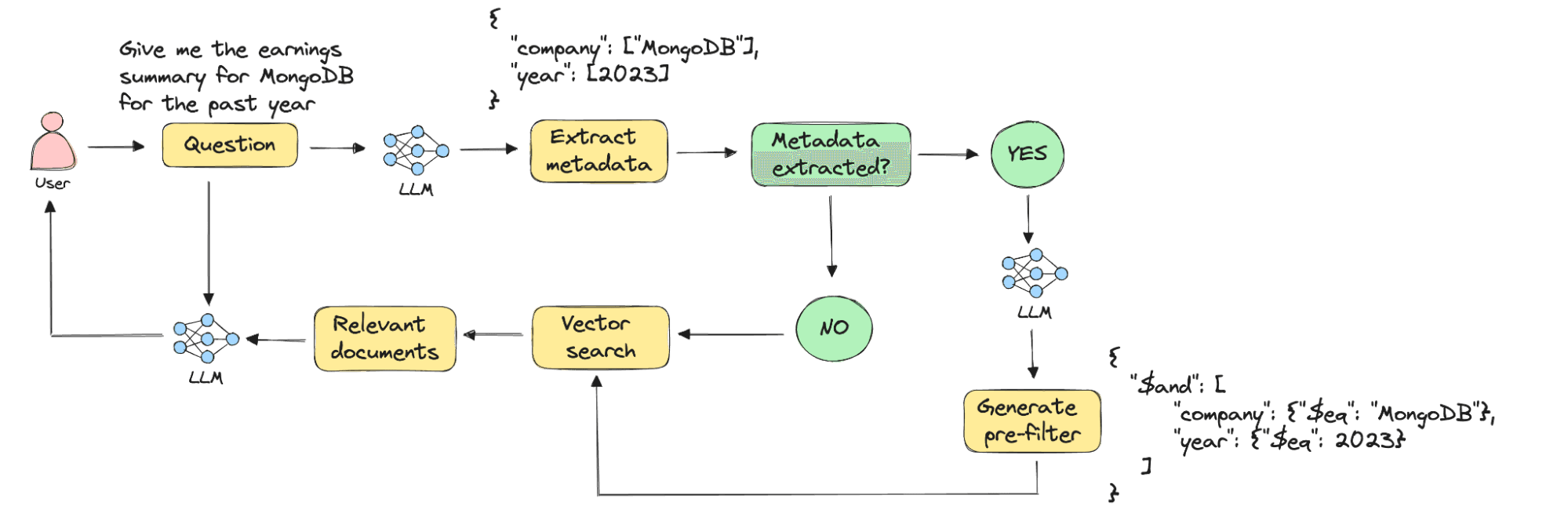
Given a user question, an LLM first tries to extract metadata from it according to a specified metadata schema. If the specified metadata is found, an LLM generates a filter definition that gets applied as a pre-filter during vector search. Otherwise, the user query alone is used to retrieve results using vector search. Finally, the retrieved context and user question, along with any other prompts, are passed to an LLM to generate an answer.
We will use 10-K filings from 30 Fortune 500 companies — the raw PDFs are available in a Google Drive folder. These reports, required by the U.S. Securities and Exchange Commission (SEC), offer a deep dive into a company's financial performance, including financial history, statements, earnings per share, and other crucial data points. For investors, 10-Ks are invaluable tools for making informed decisions. You can easily access and download these reports by visiting the website of any publicly traded US company.
We will use Unstructured to chunk, embed, and extract metadata from PDF documents and prepare them for RAG. We will use MongoDB as the vector store for our application. Finally, we will use LangGraph to orchestrate our RAG system as a stateful, DAG-like workflow.
The first step of self-querying retrieval is to decide what metadata to extract from your raw data. Doing this exercise before ingesting your data into a vector database ensures that all the required metadata is captured in the ingested documents, and the corresponding fields indexed. Not doing so beforehand can result in errors and inefficiencies downstream due to the LLM not extracting the right metadata from user queries, using wrong field names when generating the pre-filters, or querying for unindexed fields.
A good way to determine what metadata to extract is working backward from your best guess of the types of queries users might ask of your system. For our investment assistant, for example, we expect users to ask questions about specific companies and years. So this is the metadata we will start with. MongoDB’s flexible document model means you can always update existing documents with new metadata fields based on observations from real user interactions.
Vamos precisar das seguintes bibliotecas para este tutorial:
- langgraph: Python package to build stateful, multi-actor applications with LLMs
- openai: Python package to interact with OpenAI APIs
- pymongo: Python package to interact with MongoDB databases and collections
- sentence-transformers: Python package for open-source language models
- unstructured-ingest: Python package for data processing using Unstructured
1 !pip install -qU langgraph openai pymongo sentence-transformers "unstructured-ingest[pdf, s3, mongodb, embed-huggingface]"
In this tutorial, we will use Unstructured’s Serverless API to prepare our dataset for RAG. The Serverless API is a production-grade API for processing 25+ different unstructured file types, including PDFs. To use the API, first sign up for a free 14-day trial. Once you sign up, you will get access to a personalized dashboard where you will find your API key and the API endpoint URL. Set these in your code:
1 UNSTRUCTURED_API_KEY = "your-api-key" 2 UNSTRUCTURED_URL = "your-api-url"
We will use MongoDB Atlas as the vector store for our RAG application. But first, you will need a MongoDB Atlas account with a database cluster. Once you do that, you will need to get the connection string to connect to your cluster. Follow these steps to get set up:
- Obtain the connection string for your database cluster.
Once you have the connection string, set it in your code. Also, set the name of the database (
MONGODB_DB_NAME) and collection (MONGODB_COLLECTION) you want to ingest data into. Finally, instantiate the MongoDB client to connect to your database:1 # Your MongoDB connection string (uri), and collection/database names 2 MONGODB_URI = "your-mongodb-uri" 3 MONGODB_DB_NAME = "your-db-name" 4 MONGODB_COLLECTION = "your-collection-name" 5 # Instantiate the MongoDB client 6 mongodb_client = MongoClient( 7 MONGODB_URI, appname="devrel.content.selfquery_mongodb_unstructured" 8 )
Unstructured supports loading documents from over 20 different sources, including AWS S3, Azure Storage, and Google Cloud Storage. For this tutorial, we have downloaded the raw PDFs into an S3 bucket, but you can also download them to a local directory and use them as your data source.
If you are using an S3 bucket as your data source, you will need to set the S3 URI and your AWS authentication credentials in the code as well. If using a local directory as the data source, skip this step:
1 # Your AWS authentication credentials 2 AWS_KEY = "your-aws-access-key-id" 3 AWS_SECRET = "your-aws-secret-access-key" 4 # S3 URI for the Access Point to the bucket with PDF files 5 AWS_S3_NAME = ""
Let’s also specify the embedding model and LLM to use:
1 # Embedding model to use 2 EMBEDDING_MODEL_NAME = "BAAI/bge-base-en-v1.5" 3 # Completion model to use 4 COMPLETION_MODEL_NAME = "gpt-4o-2024-08-06"
We will use BAAI’s open-source bge-base-en-v1.5 embedding model from Hugging Face. The model produces embeddings with 768 dimensions. As for the LLM, we will use the latest version of GPT-4o throughout the tutorial.
Now that we have set all our prerequisites, let’s define a PDF processing pipeline using the unstructured-ingest library.
1 from unstructured_ingest.v2.pipeline.pipeline import Pipeline 2 from unstructured_ingest.v2.interfaces import ProcessorConfig 3 from unstructured_ingest.v2.processes.partitioner import PartitionerConfig 4 from unstructured_ingest.v2.processes.chunker import ChunkerConfig 5 from unstructured_ingest.v2.processes.embedder import EmbedderConfig 6 from unstructured_ingest.v2.processes.connectors.fsspec.s3 import ( 7 S3ConnectionConfig, 8 S3DownloaderConfig, 9 S3IndexerConfig, 10 S3AccessConfig, 11 ) 12 from unstructured_ingest.v2.processes.connectors.local import LocalUploaderConfig 13 14 WORK_DIR = "/content/temp" 15 16 Pipeline.from_configs( 17 context=ProcessorConfig( 18 verbose=True, tqdm=True, num_processes=5, work_dir=WORK_DIR 19 ), 20 indexer_config=S3IndexerConfig(remote_url=AWS_S3_NAME), 21 downloader_config=S3DownloaderConfig(), 22 source_connection_config=S3ConnectionConfig( 23 access_config=S3AccessConfig(key=AWS_KEY, secret=AWS_SECRET) 24 ), 25 partitioner_config=PartitionerConfig( 26 partition_by_api=True, 27 api_key=UNSTRUCTURED_API_KEY, 28 partition_endpoint=UNSTRUCTURED_URL, 29 strategy="hi_res", 30 additional_partition_args={ 31 "split_pdf_page": True, 32 "split_pdf_allow_failed": True, 33 "split_pdf_concurrency_level": 15, 34 }, 35 ), 36 chunker_config=ChunkerConfig( 37 chunking_strategy="by_title", 38 chunk_max_characters=1500, 39 chunk_overlap=150, 40 ), 41 embedder_config=EmbedderConfig( 42 embedding_provider="langchain-huggingface", 43 embedding_model_name=EMBEDDING_MODEL_NAME, 44 ), 45 uploader_config=LocalUploaderConfig(output_dir="/content/ingest-outputs"), 46 ).run()
The pipeline above is constructed from multiple configs that define different aspects of its behavior:
- ProcessorConfig: This defines the general parameters of the pipeline's behavior such as logging, cache location (this one is important in this example), re-processing, etc.
- S3IndexerConfig, S3DownloaderConfig, e S3ConnectionConfig: These are the configs for the AWS S3 source connector.
- PartitionerConfig: This partitions the documents into standardized JSON containing document elements and metadata. The
hi_resstrategy means that the Unstructured API will employ OCR, document understanding models, and classical ML methods to extract and classify document elements. This strategy is recommended for complex PDFs that contain more than just text, e.g. tables and images. Learn more about partitioning strategies. - ChunkerConfig: Once all of the documents are partitioned, the next step is to chunk them. The parameters in this config control the chunking behavior. We use the
by_titlechunking strategy to keep document sections together until the chunk size (chunk_max_characters) is reached. We specify achunk_overlapto maintain continuity at the chunk boundaries. - EmbedderConfig: The final processing step is to embed the chunks. We will use the
bge-base-en-v1.5model via thelangchain-huggingfaceintegration. - LocalUploaderConfig: This config allows us to store the final results locally in the specified directory.
Once the pipeline finishes running, we will have the final results in
*.json files in the /content/ingest-outputs local directory, as well as cached results for each of the pipeline steps in the WORK_DIR directory.If using a local directory as the data source, uncomment the local connector imports and configs in the code and comment out the S3 connector imports and configs instead.
In this step, we want to add the company name and fiscal year as custom metadata to each chunk, to enable pre-filtering during vector search. Luckily, the Form-10K documents have a more or less standard page with this information, so we can use simple regular expressions (regex) to extract the required metadata from them.
Let’s first define a function to extract the year:
1 def get_fiscal_year(elements: dict) -> int: 2 # Regular expression pattern to find the element containing the fiscal year 3 pattern = r"for the (fiscal\s+)?year ended.*?(\d{4})" 4 year = 0 5 for i in range(len(elements)): 6 match = re.search(pattern, elements[i]["text"], re.IGNORECASE) 7 if match: 8 year = match.group(0)[-4:] 9 try: 10 year = int(year) 11 except: 12 year = 0 13 return year
The Form-10K documents are filed for a specific fiscal year, and there’s a standard sentence in each document that indicates what year the document was filed for, e.g., “For the fiscal year ended December 31, 2023.” The function above takes the elements of a document as input, uses a regex to find the line containing the filing date, and extracts the year from this line. We return the year as
int to be able to leverage comparison operators later.Let’s define another function to extract the company name:
1 def get_company_name(elements: dict) -> str: 2 name = "" 3 # In most cases the name of the company is right before/above the following line 4 substring = "(Exact name of registrant as specified" 5 for i in range(len(elements)): 6 if substring.lower() in elements[i]["text"].lower(): 7 pattern = ( 8 r"([A-Z][A-Za-z\s&.,]+?)\s*\(Exact name of registrant as specified" 9 ) 10 match = re.search(pattern, elements[i]["text"], re.IGNORECASE) 11 if match: 12 name = match.group(1).strip() 13 name = name.split("\n\n")[-1] 14 15 if name == "": 16 for i in range(len(elements)): 17 # In some cases, the name of the company is right after/below the following line 18 match = re.search( 19 r"Exact name of registrant as specified in its charter:\n\n(.*?)\n\n", 20 elements[i]["text"], 21 ) 22 if match: 23 name = match.group(1) 24 else: 25 # In other cases, the name follows the "Commission File Number [Number]" line 26 match = re.search( 27 r"Commission File Number.*\n\n(.*?)\n\n", elements[i]["text"] 28 ) 29 if match: 30 name = match.group(1) 31 return name
Extracting the company name is similar to how we extracted the fiscal year, except there is a little more variation in where exactly the company name is mentioned in the document, so we employ multiple regex expressions. In most cases, you will find the company name right after the line, “Exact name of registrant as specified.” However, in some cases, the company name precedes this line or follows the “Commission File Number [Number]” instead.
Now, let’s walk through the directory with the embedding results, and for each document, find the company name and year and add them as custom metadata to all elements of the document:
1 directory = f"{WORK_DIR}/embed" 2 3 for filename in os.listdir(directory): 4 if filename.endswith(".json"): 5 file_path = os.path.join(directory, filename) 6 print(f"Processing file {filename}") 7 try: 8 with open(file_path, "r") as file: 9 data = json.load(file) 10 11 company_name = get_company_name(data) 12 fiscal_year = get_fiscal_year(data) 13 14 # Add custom metadata fields to each entry 15 for entry in data: 16 entry["metadata"]["custom_metadata"] = {} 17 entry["metadata"]["custom_metadata"]["company"] = company_name 18 entry["metadata"]["custom_metadata"]["year"] = fiscal_year 19 20 with open(file_path, "w") as file: 21 json.dump(data, file, indent=2) 22 23 print(f"Successfully updated {file_path} with custom metadata fields.") 24 except json.JSONDecodeError as e: 25 print(f"Error parsing JSON in {file_path}: {e}") 26 except IOError as e: 27 print(f"Error reading from or writing to {file_path}: {e}")
The code above reads
*.json files from the working directory that contains the results of the embedding step of the pipeline. Each file is the result of processing a single document, so you have one JSON file for each original PDF document. For each file, we’re using the previously defined functions to extract the fiscal date and company name and add these values as custom metadata fields to all of the document elements. We then write the results back to the original file.To write the final processed documents to MongoDB, we will need to re-run the pipeline we defined in Step 4, except we will now change the destination from local to MongoDB.
1 from unstructured_ingest.v2.processes.connectors.mongodb import ( 2 MongoDBConnectionConfig, 3 MongoDBUploadStagerConfig, 4 MongoDBUploaderConfig, 5 MongoDBAccessConfig, 6 ) 7 8 Pipeline.from_configs( 9 context=ProcessorConfig( 10 verbose=True, tqdm=True, num_processes=5, work_dir=WORK_DIR 11 ), 12 indexer_config=S3IndexerConfig(remote_url=AWS_S3_NAME), 13 downloader_config=S3DownloaderConfig(), 14 source_connection_config=S3ConnectionConfig( 15 access_config=S3AccessConfig(key=AWS_KEY, secret=AWS_SECRET) 16 ), 17 partitioner_config=PartitionerConfig( 18 partition_by_api=True, 19 api_key=UNSTRUCTURED_API_KEY, 20 partition_endpoint=UNSTRUCTURED_URL, 21 strategy="hi_res", 22 additional_partition_args={ 23 "split_pdf_page": True, 24 "split_pdf_allow_failed": True, 25 "split_pdf_concurrency_level": 15, 26 }, 27 ), 28 chunker_config=ChunkerConfig( 29 chunking_strategy="by_title", 30 chunk_max_characters=1500, 31 chunk_overlap=150, 32 ), 33 embedder_config=EmbedderConfig( 34 embedding_provider="langchain-huggingface", 35 embedding_model_name=EMBEDDING_MODEL_NAME, 36 ), 37 destination_connection_config=MongoDBConnectionConfig( 38 access_config=MongoDBAccessConfig(uri=MONGODB_URI), 39 collection=MONGODB_COLLECTION, 40 database=MONGODB_DB_NAME, 41 ), 42 stager_config=MongoDBUploadStagerConfig(), 43 uploader_config=MongoDBUploaderConfig(batch_size=100), 44 ).run()
The pipeline above is the same as we had in Step 4, the only difference being the destination location for the data processing results, which is now the MongoDB collection specified in Step 2. The MongoDB destination is set up using three configurations:
MongoDBConnectionConfig, MongoDBUploadStagerConfig, e MongoDBUploaderConfig. These configurations establish the connection to our MongoDB Atlas database, specify where the data needs to be uploaded, and note any additional upload parameters such as batch_size to bulk ingest the data into MongoDB.An example document ingested into MongoDB is as follows:
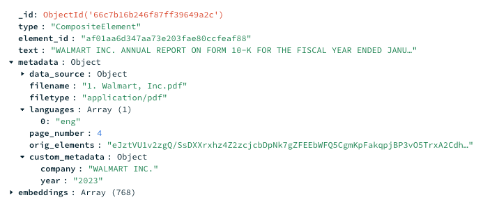
Note the custom metadata fields
metadata.custom_metadata.company and metadata.custom_metadata.year containing the company name and year that the document was published in.As mentioned previously, we will use LangGraph to orchestrate our RAG system. LangGraph allows you to build LLM systems as graphs. The nodes of the graph are functions or tools to perform specific tasks, while the edges define routes between nodes — these can be fixed, conditional, or even cyclic. Each graph has a state which is a shared data structure that all the nodes can access and make updates to. You can define custom attributes within the state depending on what parameters you want to track across the nodes of the graph.
Let’s go ahead and define the state of our graph:
1 class GraphState(TypedDict): 2 """ 3 Represents the state of the graph. 4 5 Attributes: 6 question: User query 7 metadata: Extracted metadata 8 filter: Filter definition 9 documents: List of retrieved documents from vector search 10 memory: Conversational history 11 """ 12 13 question: str 14 metadata: Dict 15 filter: Dict 16 context: List[str] 17 memory: Annotated[list, add_messages]
O código acima:
- Creates a
GraphStateclass that represents the state of the graph for our assistant. - Defines the state schema using the
TypedDictmodel to create type-safe dictionaries that can help catch errors at compile-time rather than runtime. - Annotates the
memorykey in the state with theadd_messagesreducer function, telling LangGraph to append new messages to the existing list, rather than overwriting it.
Next, let’s define the nodes of our graph. Nodes contain the main logic of the system. They are essentially Python functions and may or may not use an LLM. Each node takes the graph
state as input, performs some computation, and returns an updated state.Our assistant has four main functionalities:
- Extract metadata from a natural language query.
- Generate a MongoDB Query API filter definition.
- Retrieve documents from MongoDB using semantic search.
- Generate an answer to the user's question.
Let’s define nodes for each of the above functionalities.
For our assistant, extracting metadata in a specific format is crucial to avoid errors and incorrect results downstream. OpenAI recently released Structured Outputs, a feature that ensures their models will always generate responses that adhere to a specified schema. Let’s try this out!
Let’s create a Pydantic model that defines the metadata schema:
1 class Metadata(BaseModel): 2 """Metadata to use for pre-filtering.""" 3 4 company: List[str] = Field(description="List of company names") 5 year: List[str] = Field(description="List containing start year and end year")
In the above code, we create a Pydantic model called
Metadata with company and year as attributes. Each attribute is of type List[str], indicating a list of strings.Now, let’s define a function to extract metadata from the user question:
1 def extract_metadata(state: Dict) -> Dict: 2 """ 3 Extract metadata from natural language query. 4 5 Args: 6 state (Dict): The current graph state 7 8 Returns: 9 Dict: New key added to state i.e. metadata containing the metadata extracted from the user query. 10 """ 11 print("---EXTRACTING METADATA---") 12 question = state["question"] 13 system = f"""Extract the specified metadata from the user question: 14 - company: List of company names, eg: Google, Adobe etc. Match the names to companies on this list: {companies} 15 - year: List of [start year, end year]. Guidelines for extracting dates: 16 - If a single date is found, only include that. 17 - For phrases like 'in the past X years/last year', extract the start year by subtracting X from the current year. The current year is {datetime.now().year}. 18 - If more than two dates are found, only include the smallest and the largest year.""" 19 completion = openai_client.beta.chat.completions.parse( 20 model=COMPLETION_MODEL_NAME, 21 messages=[ 22 {"role": "system", "content": system}, 23 {"role": "user", "content": question}, 24 ], 25 response_format=Metadata, 26 ) 27 result = completion.choices[0].message.parsed 28 # If no metadata is extracted return an empty dictionary 29 if len(result.company) == 0 and len(result.year) == 0: 30 return {"metadata": {}} 31 metadata = { 32 "metadata.custom_metadata.company": result.company, 33 "metadata.custom_metadata.year": result.year, 34 } 35 return {"metadata": metadata}
O código acima:
- Gets the user question from the graph state (
state). - Defines a system prompt instructing the LLM to extract company names and date ranges from the question. We specifically ask the LLM to match company names to the list of companies in our dataset. Otherwise, the pre-filter won’t match any records in our knowledge base.
- Passes the
MetadataPydantic model as theresponse_formatargument to theparse()method of OpenAI’s Chat Completions API to get the LLM’s response back as aMetadataobject. - Sets the
metadataattribute of the graphstateto{}, if no metadata is extracted by the LLM. - Sets the
metadataattribute to a dictionary consisting of keys corresponding to metadata fields in our MongoDB documents — i.e.,metadata.custom_metadata.companyandmetadata.custom_metadata.year— and values obtained from the LLM’s response, if metadata is found.
Next, let’s define a function to generate the filter definition:
1 def generate_filter(state: Dict) -> Dict: 2 """ 3 Generate MongoDB Query API filter definition. 4 5 Args: 6 state (Dict): The current graph state 7 8 Returns: 9 Dict: New key added to state i.e. filter. 10 """ 11 print("---GENERATING FILTER DEFINITION---") 12 metadata = state["metadata"] 13 system = """Generate a MongoDB filter definition from the provided fields. Follow the guidelines below: 14 - Respond in JSON with the filter assigned to a `filter` key. 15 - The field `metadata.custom_metadata.company` is a list of companies. 16 - The field `metadata.custom_metadata.year` is a list of one or more years. 17 - If any of the provided fields are empty lists, DO NOT include them in the filter. 18 - If both the metadata fields are empty lists, return an empty dictionary {{}}. 19 - The filter should only contain the fields `metadata.custom_metadata.company` and `metadata.custom_metadata.year` 20 - The filter can only contain the following MongoDB Query API match expressions: 21 - $gt: Greater than 22 - $lt: Lesser than 23 - $gte: Greater than or equal to 24 - $lte: Less than or equal to 25 - $eq: Equal to 26 - $ne: Not equal to 27 - $in: Specified field value equals any value in the specified array 28 - $nin: Specified field value is not present in the specified array 29 - $nor: Logical NOR operation 30 - $and: Logical AND operation 31 - $or: Logical OR operation 32 - If the `metadata.custom_metadata.year` field has multiple dates, create a date range filter using expressions such as $gt, $lt, $lte and $gte 33 - If the `metadata.custom_metadata.company` field contains a single company, use the $eq expression 34 - If the `metadata.custom_metadata.company` field contains multiple companies, use the $in expression 35 - To combine date range and company filters, use the $and operator 36 """ 37 completion = openai_client.chat.completions.create( 38 model=COMPLETION_MODEL_NAME, 39 temperature=0, 40 messages=[ 41 {"role": "system", "content": system}, 42 {"role": "user", "content": f"Fields: {metadata}"}, 43 ], 44 response_format={"type": "json_object"}, 45 ) 46 result = json.loads(completion.choices[0].message.content) 47 return {"filter": result.get("filter", {})}
O código acima:
- Extracts metadata from the graph state.
- Defines a system prompt containing instructions on how to create the filter definition — match expressions and operators supported, fields to use, etc.
- Gets the output of the specified LLM as a JSON object by passing
json_objectas theresponse_formatargument to the Chat Completions API call as well as specifying the wordJSONin the system prompt. - Sets the
filterattribute of the graph state to the generated filter definition.
The next step is to define a graph node that retrieves documents from MongoDB using semantic search. But first, you will need to create a vector search index:
1 collection = mongodb_client[MONGODB_DB_NAME][MONGODB_COLLECTION] 2 VECTOR_SEARCH_INDEX_NAME = "vector_index" 3 4 model = { 5 "name": VECTOR_SEARCH_INDEX_NAME, 6 "type": "vectorSearch", 7 "definition": { 8 "fields": [ 9 { 10 "type": "vector", 11 "path": "embeddings", 12 "numDimensions": 768, 13 "similarity": "cosine", 14 }, 15 {"type": "filter", "path": "metadata.custom_metadata.company"}, 16 {"type": "filter", "path": "metadata.custom_metadata.year"}, 17 ] 18 }, 19 } 20 collection.create_search_index(model=model)
O código acima:
- Specifies the collection to perform semantic search against.
- Specifies the name of the vector search index.
- Specifies the vector search index definition which contains the path to the embeddings field in the documents (
path), the number of embedding dimensions (numDimensions), the similarity metric to find nearest neighbors (similarity), and the path to the filter fields to index. - Creates the vector search index.
Now, let’s define a function that performs vector search:
1 def vector_search(state: Dict) -> Dict: 2 """ 3 Get relevant information using MongoDB Atlas Vector Search 4 5 Args: 6 state (Dict): The current graph state 7 8 Returns: 9 Dict: New key added to state i.e. documents. 10 """ 11 print("---PERFORMING VECTOR SEARCH---") 12 question = state["question"] 13 filter = state["filter"] 14 # We always want a valid filter object 15 if not filter: 16 filter = {} 17 query_embedding = embedding_model.encode(question).tolist() 18 pipeline = [ 19 { 20 "$vectorSearch": { 21 "index": VECTOR_SEARCH_INDEX_NAME, 22 "path": "embeddings", 23 "queryVector": query_embedding, 24 "numCandidates": 150, 25 "limit": 5, 26 "filter": filter, 27 } 28 }, 29 { 30 "$project": { 31 "_id": 0, 32 "text": 1, 33 "score": {"$meta": "vectorSearchScore"}, 34 } 35 }, 36 ] 37 # Execute the aggregation pipeline 38 results = collection.aggregate(pipeline) 39 # Drop documents with cosine similarity score < 0.8 40 relevant_results = [doc["text"] for doc in results if doc["score"] >= 0.8] 41 context = "\n\n".join([doc for doc in relevant_results]) 42 return {"context": context}
O código acima:
- Reads the user question and filter definition from the graph state.
- Sets it to an empty object, if no filter is found. Remember, we skip directly to vector search if no metadata is extracted.
- Embeds the user query using the
bge-base-en-v1.5model. - Creates and runs an aggregation pipeline to perform semantic search. The
$vectorSearchstage retrieves documents using nearest neighbor search — thenumCandidatesfield indicates how many nearest neighbors to consider, thelimitfield indicates how many documents to return, and thefilterfield specifies the pre-filters. The$projectstage that follows outputs only the specified fields — i.e.,textand the vector search similarity score from the returned documents. - Filters out documents with a similarity score of < 0.8 to ensure only highly relevant documents are returned.
- Concatenates the
textfield values from the final list of documents into a string and sets it as thecontextattribute of the graph state.
Let’s define the final node in our graph to generate answers to questions.
1 def generate_answer(state: Dict) -> Dict: 2 """ 3 Generate the final answer to the user query 4 5 Args: 6 state (Dict): The current graph state 7 8 Returns: 9 Dict: New key added to state i.e. generation. 10 """ 11 print("---GENERATING THE ANSWER---") 12 question = state["question"] 13 context = state["context"] 14 memory = state["memory"] 15 system = f"Answer the question based only on the following context. If the context is empty or if it doesn't provide enough information to answer the question, say I DON'T KNOW" 16 completion = openai_client.chat.completions.create( 17 model=COMPLETION_MODEL_NAME, 18 temperature=0, 19 messages=[ 20 {"role": "system", "content": system}, 21 { 22 "role": "user", 23 "content": f"Context:\n{context}\n\n{memory}\n\nQuestion:{question}", 24 }, 25 ], 26 ) 27 answer = completion.choices[0].message.content 28 return {"memory": [HumanMessage(content=context), AIMessage(content=answer)]}
O código acima:
- Reads the user question, context retrieved from vector search, and any conversational history from the graph state.
- Defines a system prompt to instruct the LLM to only answer based on the provided context. This is a simple step to mitigate hallucinations.
- Passes the system prompt, retrieved context, chat history, and user question to OpenAI’s Chat Completions API to get back a response from the specified LLM.
- Updates the memory attribute of the graph state by adding the retrieved context and LLM response to the existing list of messages.
As mentioned previously, edges in a LangGraph graph define interactions between nodes. Our graph mostly has fixed edges between nodes, except one conditional edge to skip filter generation and go directly to vector search based on whether or not metadata was extracted from the user query.
Let’s define the logic for this conditional edge:
1 def check_metadata_extracted(state: Dict) -> str: 2 """ 3 Check if any metadata is extracted. 4 5 Args: 6 state (Dict): The current graph state 7 8 Returns: 9 str: Binary decision for next node to call 10 """ 11 12 print("---CHECK FOR METADATA---") 13 metadata = state["metadata"] 14 # If no metadata is extracted, skip the generate filter step 15 if not metadata: 16 print("---DECISION: SKIP TO VECTOR SEARCH---") 17 return "vector_search" 18 # If metadata is extracted, generate filter definition 19 else: 20 print("---DECISION: GENERATE FILTER---") 21 return "generate_filter"
In the above code, we extract the metadata attribute of the graph state. If no metadata is found, it returns the string “vector_search.” If not, it returns the string “generate_filter.” We will see how to tie the outputs of this routing function to nodes in the next step.
Finally, let’s build the graph by connecting the nodes using edges.
1 from langgraph.graph import END, StateGraph, START 2 from langgraph.checkpoint.memory import MemorySaver 3 from IPython.display import Image, display 4 5 workflow = StateGraph(GraphState) 6 # Adding memory to the graph 7 memory = MemorySaver() 8 9 # Add nodes 10 workflow.add_node("extract_metadata", extract_metadata) 11 workflow.add_node("generate_filter", generate_filter) 12 workflow.add_node("vector_search", vector_search) 13 workflow.add_node("generate_answer", generate_answer) 14 15 # Add edges 16 workflow.add_edge(START, "extract_metadata") 17 workflow.add_conditional_edges( 18 "extract_metadata", 19 check_metadata_extracted, 20 { 21 "vector_search": "vector_search", 22 "generate_filter": "generate_filter", 23 }, 24 ) 25 workflow.add_edge("generate_filter", "vector_search") 26 workflow.add_edge("vector_search", "generate_answer") 27 workflow.add_edge("generate_answer", END) 28 29 # Compile the graph 30 app = workflow.compile(checkpointer=memory)
O código acima:
- Instantiates the graph using the
StateGraphclass and parameterizes it with the graph state defined in Step 7. - Initializes an in-memory checkpointer using the
MemorySaver()class. Checkpointers persist the graph state between interactions in LangGraph. This is how our RAG system persists chat history. - Adds all the nodes defined in Step 8 to the graph using the
add_nodemethod. The first argument toadd_nodeis the name of the node and the second argument is the Python function corresponding to the node. - Adds fixed edges using the
add_edgemethod. Notice the edges betweenSTARTandextract_metadata, egenerate_answerandEND.STARTandENDare special nodes to indicate which node to call first and which nodes have no following actions. - Adds conditional edges from the
extract_metadatanode to thegenerate_filterandvector_searchnodes based on the outputs of the routing function defined in Step 9. - Compiles the graph with the memory checkpointer.
We can visualize our graph as a Mermaid diagram. This helps to verify the nodes and edges, especially for complicated workflows.
1 try: 2 display(Image(app.get_graph().draw_mermaid_png())) 3 except Exception: 4 # This requires some extra dependencies and is optional 5 pass
In the above code, we use the
get_graph() method to get the compiled graph and the draw_mermaid_png method to generate a Mermaid diagram of the graph as a PNG image.Here’s what our graph looks like:

As the last step, let’s define a function that takes user input and streams the outputs of the graph execution back to the user.
1 def execute_graph(thread_id: str, question: str) -> None: 2 """ 3 Execute the graph and stream its output 4 5 Args: 6 thread_id (str): Conversation thread ID 7 question (str): User question 8 """ 9 # Add question to the question and memory attributes of the graph state 10 inputs = {"question": question, "memory": [HumanMessage(content=question)]} 11 config = {"configurable": {"thread_id": thread_id}} 12 # Stream outputs as they come 13 for output in app.stream(inputs, config): 14 for key, value in output.items(): 15 print(f"Node {key}:") 16 print(value) 17 print("---FINAL ANSWER---") 18 print(value["memory"][-1].content)
O código acima:
- Takes the user question (
question) and thread ID (thread_id) as input. - Creates an
inputsdictionary containing the initial updates to the graph state. In our case, we want to add the user question to thequestionandmemoryattributes of the graph state. - Creates a runtime config containing the input thread ID. Thread IDs are unique IDs assigned to memory checkpoints in LangGraph. Each checkpoint has a separate state.
- Streams the outputs of the graph, specifically the node names and outputs.
- Prints the final answer from the system, extracted from the return value of the last node in the graph — i.e. the
generate_answernode.
An example run of the system looks as follows:
1 execute_graph("1", "Sales summary for Walmart for 2023.") 2 3 ---EXTRACTING METADATA--- 4 ---CHECK FOR METADATA--- 5 ---DECISION: GENERATE FILTER--- 6 'Node extract_metadata:' 7 {'metadata': {'metadata.custom_metadata.company': ['WALMART INC.'], 'metadata.custom_metadata.year': ['2023']}} 8 ---GENERATING FILTER DEFINITION--- 9 'Node generate_filter:' 10 {'filter': {'$and': [{'metadata.custom_metadata.company': {'$eq': 'WALMART INC.'}}, {'metadata.custom_metadata.year': {'$eq': 2023}}]}} 11 ---PERFORMING VECTOR SEARCH--- 12 'Node vector_search:' 13 {'context': 'DOCUMENTS INCORPORATED BY REFERENCE...'} 14 ---GENERATING THE ANSWER--- 15 'Node generate_answer:' 16 {'memory': [HumanMessage(content='DOCUMENTS INCORPORATED BY REFERENCE...'), AIMessage(content='In fiscal 2023, Walmart generated total revenues of $611.3 billion, primarily comprised of net sales amounting to $605.9 billion. Walmart International contributed $101.0 billion to the fiscal 2023 consolidated net sales, representing 17% of the total.')]} 17 ---FINAL ANSWER--- 18 In fiscal 2023, Walmart generated total revenues of $611.3 billion, primarily comprised of net sales amounting to $605.9 billion. Walmart International contributed $101.0 billion to the fiscal 2023 consolidated net sales, representing 17% of the total.
Let’s ask a follow-up question to ensure that the graph persists chat history:
1 execute_graph("1", "What did I just ask you?") 2 3 ---EXTRACTING METADATA--- 4 ---CHECK FOR METADATA--- 5 ---DECISION: SKIP TO VECTOR SEARCH--- 6 'Node extract_metadata:' 7 {'metadata': {}} 8 ---PERFORMING VECTOR SEARCH--- 9 'Node vector_search:' 10 {'context': ''} 11 ---GENERATING THE ANSWER--- 12 'Node generate_answer:' 13 {'memory': [HumanMessage(content=''), AIMessage(content='You asked for the sales summary for Walmart for 2023.')]} 14 ---FINAL ANSWER--- 15 You asked for the sales summary for Walmart for 2023.
The system was able to recall what we asked previously.
There you go! We have successfully built a RAG system with self-querying retrieval and memory.
In this tutorial, we learned how to build an advanced RAG system that leverages self-querying retrieval. These techniques are useful in scenarios where user queries might contain important keywords that embeddings might not capture. We built an investment assistant that extracts company names and date ranges from user queries, uses them to generate MongoDB filter definitions, and applies them as pre-filters during vector search to get the most accurate information for an LLM to answer questions about the financial performance of specific companies during certain time periods.
For more advanced content, such as building agentic systems, check out the following tutorials on our Developer Center:
Principais comentários nos fóruns

Avaliar este tutorial
Relacionado
Artigo
Comparação de técnicas de NLP para Atlas Search de produtos escaláveis
Sep 23, 2024 | 8 min read
Tutorial
Como escolher o melhor modelo de incorporação para seu aplicativo LLM
Nov 07, 2024 | 16 min read
oooh … gotta do this one … brb