How Columnar Storage in Time Series Collection Delivers Real Cost Savings

A sensor measuring temperatures once a second generates 86,400 readings each day. Normally, every reading is stored in a full document structure even when the temperature changes by a tenth of a degree, or the loss value shifts by 0.001. But for time series workloads—whether IoT sensors or AI training pipelines—it's quietly expensive. And it gets worse the more data you retain.

Time Series Collections were designed specifically to handle these massive streams of timestamped measurements with shared metadata and evolving schemas. Instead of treating each document as an independent record, they recognize what time series data actually is: a highly repetitive structure with slowly changing values.

In this blog post, we’ll explore how we introduced columnar-style efficiency while preserving the flexible document model and how it can benefit customer use-cases.

Problems with row-based storage

Consider millions of temperature readings from a single device. The temperature drifts by fractions of a degree. Maybe it doesn't change at all. In a traditional row-based storage engine, every record is stored whole—the object structure, the device ID, the timestamp format, the field names over and over.

This can severely compound as the core unit of storage is a flexible, self-describing BSON document. When a new reading arrives, the entire object gets written—timestamp, device ID, field definitions, data types and finally the actual value. 

• Metadata and structure: field names, types, object shape

• Static fields: device ID, location, anything that rarely changes

• Redundant precision: full absolute values when only deltas matter

This can be incredibly inefficient for data streams where the schema is constant, but the values are highly correlated. 

Let’s look at how Time Series Collections solve these problems.

Metadata deduplication

The first optimization is straightforward but very impactful—stop storing field names millions of times.

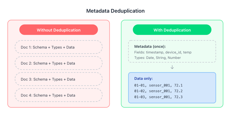
Instead of each document carrying its own schema definition—since all documents coming from particular deviceID share the same schema (i.e., they are all temperature readings from the same type of device), the database stores the BSON field names, data types, and internal object structure only once for the entire group of documents, not once per document.

For high-frequency ingestion, this alone can cut storage significantly. 

Hybrid columnar grouping for documents

With structural redundancy eliminated, the next part is enabling the columnar structure needed for advanced compression.Time Series Collections solve this by shifting from row-oriented to logically columnar storage without forcing you into a rigid schema.

Two parameters do most of the work to define this columnar data structure:

• metaField: all documents sharing the same metaField value (and falling within the same time window) can be grouped together for better colocation. Instead of storing data record-by-record, the system groups identical fields across hundreds of documents into columns. You're no longer looking at one temperature reading inside an entire document—you're looking at a sequential stream of temperature values, stripped of redundant structure.

• Granularity: which helps define how frequently data arrives (e.g., hours or minutes). By choosing the granularity that best matches the time span between consecutive measurements for the same metaField, you tell the system to create internal grouping sizes that suit your use-case. Match this to your actual ingestion pattern and you help the engine pack store documents efficiently.

Combined, this means that instead of treating every BSON document as an independent record, the system treats all documents with the same metaField as belonging to a single, compressible stream of data. This fundamental transformation sets the stage for the powerful compression techniques we'll explore next.

Figure 1. Metadata deduplication.

Column compression

Once values are stripped of metadata and the columnar grouping, the system can apply value-based encoding techniques that exploit the patterns inherent in time series data.

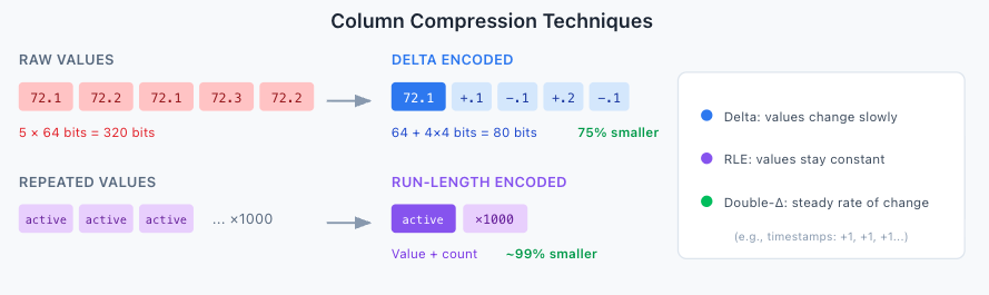
1. Delta encoding: Time series values often change by tiny amounts. Instead of storing the full value (e.g., 72.1, 72.2, 72.1), the system stores the initial value and then only the difference, or delta (e.g., 72.1, +0.1, -0.1). Since these deltas are often small, they require far fewer bits to store, and this applies to small strings, objectID etc as well.

2. Run-length encoding (RLE): If a sensor reading stays constant for many measurements (e.g., status: active, active, active, active), RLE stores the value once and counts the consecutive repetitions, dramatically shrinking the data size.

If you simply insert these documents into a regular collection or use the bucketing pattern, neither of these techniques work because of the nature of row-based data storage. The columnar arrangement is a prerequisite.

Figure 2. Column compression techniques.

What about nested documents?

Here's where Time Series Collections really shine: you don't have to flatten your data model to get great compression. The columnar compression works on nested objects at any depth, treating each unique scalar field path as its own independent column.

Consider a document with nested measurements:

You might expect that nesting breaks columnar compression—that readings would compress as a single blob, losing per-field benefits. That's not what happens.

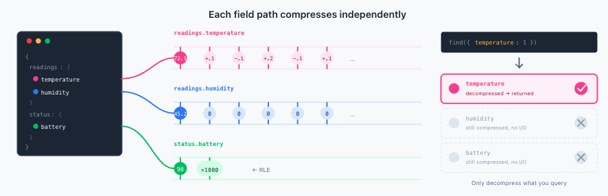
The compression algorithm treats each unique field path as an independent column. readings.temperature, readings.humidity, and readings.pressure each get their own compression stream. This means:

• If temperature fluctuates constantly but humidity stays flat, each compresses optimally for its own pattern

• A field like status.battery that changes once an hour compresses beautifully with RLE, independent of high-frequency fields

You get the same compression quality as if you'd flattened everything to the top level—but with the organizational benefits of nested structures. And this works at any nesting depth. Every unique field path becomes its own column, giving you the full richness of the document model without sacrificing storage efficiency.

Figure 3. Column compression on metrics.

Query-path benefits

Per-field columnar storage pays off at read time too. If a query only references readings.temperature, the system decompresses just that column. The humidity, pressure, and status fields stay compressed. This block processing optimization, introduced in MongoDB 8.0, means your analytical queries run faster because they're not wasting cycles decompressing data they'll never use. The queries operate directly on top of column compressed data leading low I/O and resource utilization. For dashboards scanning weeks of data or batch jobs crunching months of metrics, this adds up fast.

Practical guidelines

There are some guidelines and best practices to keep in mind as you design your workload for Time Series Collections:

• Missing fields are fine. The system handles sparse data gracefully {a: 1, b: 2} followed by {a: 1} compresses well. You should not pad documents with nulls. Just keep the fields that are present in consistent order.

• Structure for access patterns. Since each field path compresses independently, organize your documents based on how you'll query them:

• Group related measurements that you'll often query together

• Use meaningful nesting that reflects your domain model

• Don't flatten unnecessarily—the compression doesn't penalize nesting

• Match granularity to your data. If your sensors report every second, don't set granularity to hours. If they report hourly, don't set it to seconds. Granularity should match the scale of data frequency of your use-case.

Columnar compression in action

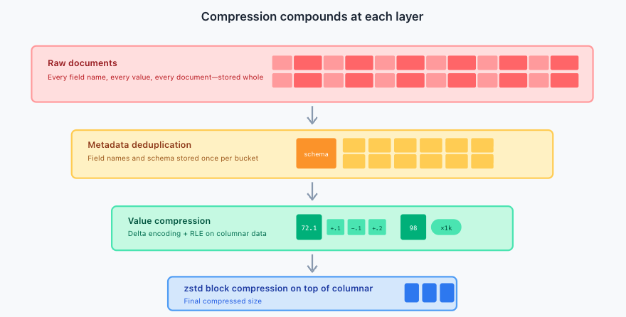
The combination of metadata deduplication, columnar arrangement, and value encoding compounds. Terabytes can collapse to gigabytes—not through lossy compression or aggressive sampling, but by eliminating structural redundancy that was never carrying information in the first place. Additionally, the storage engine zstd block compressor further reduces the size of the already column-compressed data.

Figure 4. How compression compounds at each layer.

For teams storing months or years of high-frequency data, this changes the cost calculus. Retention decisions that were previously budget-constrained become feasible. Customer workloads tend to see 70-90% compression rate on their raw data due to native columnar compression. The sheer volume of time series data presents a critical challenge; you can't just throw more hardware at the problem indefinitely. True scalability demands efficiency at the architectural level. With Time Series Collections, we have intelligently transformed the flexible document model into a logically columnar structure and applied specialized BSON Column Compression which addresses the core issue of repetition head-on. 

This matters more as workloads shift. AI training pipelines, inference monitoring, reinforcement learning signals—these generate time series data at a scale that makes traditional IoT look modest. When every experiment produces millions of timestamped metrics, and you need to query across hundreds of runs to debug a regression, storage efficiency stops being a nice-to-have.

That's the point. Not compression as a feature, but compression as an enabler, making it practical to store what you'd otherwise have to discard.