Time series data captures any signal, metric, or observation whose state changes continuously over time. Infrastructure metrics, IoT sensor readings, financial market data, observability signals, and distributed system telemetry all qualify. What they share is the need to record an ordered sequence of measurements efficiently.
The challenge is doing this in a way that keeps infrastructure stable and scalable while still enabling fast, expressive queries. Time series systems must handle sustained writes, retain historical context, and support range-based analytical queries without overwhelming memory or storage. All of these demands require efficient ingestion, intelligent storage layouts, and query mechanisms optimized for time-based access patterns.
MongoDB time series collection
MongoDB is a database built for scalable, modern applications, where developers and builders are not expected to constantly worry about the limitations of the underlying infrastructure while writing application logic. Its flexible schema design and distributed architecture allow applications to evolve rapidly, handle changing data shapes, and scale seamlessly as usage grows. This philosophy extends naturally to time series workloads, where data is continuously generated over time and needs to be ingested, stored, and queried efficiently without placing undue pressure on memory, CPU, or storage. The goal is to store time series data in a way that keeps the system stable while enabling fast, time-based queries.
MongoDB time series collections achieve this through an internal bucket pattern, where individual measurements are grouped into buckets rather than being stored as standalone documents. Each bucket holds measurements that fall within a specific time range and share the same metaField (for example, a deviceId), and it is automatically closed when it reaches either a document count limit (approximately 1,000 measurements) or a size limit (around 125 KB), whichever comes first (view documentation). These buckets maintain internal metadata, including minimum and maximum timestamps and the meta value, which effectively acts like a compound index. During range-based queries, MongoDB uses this metadata to prune irrelevant buckets entirely, avoiding unnecessary reads and decompression.
Buckets are opened and closed dynamically based on data flow, allowing MongoDB to balance memory usage and overall system stability. It is important to understand that this behavior is not unique to time series collections, nor does MongoDB attempt to keep all buckets permanently resident in memory. Like any modern database, MongoDB relies on a general-purpose storage engine (WiredTiger) that manages memory through a cache, evicting data pages from RAM when they are no longer actively accessed. Open or closed time series buckets are stored on disk just like regular documents, and only the portions of data required to satisfy active reads or writes are kept in memory.
What time series collections add on top of this general database behavior is predictability and efficiency in how data is grouped. By organizing measurements into buckets with well-defined time ranges and shared metadata, MongoDB can make smarter decisions about which data needs to be read from disk and which can be skipped entirely. When a bucket is closed, it simply means that MongoDB will no longer append new measurements to it. The bucket itself is not pinned in memory, nor does it consume special resources. If a query needs data from a closed bucket, the required pages are fetched from disk into memory just like any other document, and may later be evicted again based on cache pressure. This combination of bucket lifecycle management and standard cache eviction allows MongoDB to handle sustained time series workloads without overwhelming RAM, while still delivering efficient query performance.
With this foundation in place, the next logical question is: when do these buckets close due to size, and when do they close due to time, and how does ingestion rate influence that behavior? The upcoming sections explore this question through controlled evaluations comparing high and low ingestion rates across different time series granularities.
Understanding granularity in time series collections
When creating a time series collection in MongoDB, one of the key configuration choices is granularity. Granularity defines the expected time span of a bucket, effectively guiding MongoDB on how long a bucket should remain open based on time alone. MongoDB supports three granularity levels: seconds, minutes, and hours, each corresponding to progressively larger bucket time windows. Granularity does not dictate how frequently data must be ingested. Rather, it influences how timestamps are rounded internally, and granularity defines the maximum time span a bucket is allowed to cover before it becomes eligible for closure based on time alone. However, a bucket may be closed earlier if it reaches its size limits, approximately 1,000 measurements or around 125 KB, whichever condition is met first.
Granularity acts as a time-based constraint, not a throughput constraint. A collection set to granularity: hours can still accept data every second or every 30 seconds, just as a granularity: seconds collection can accept sparse or bursty writes. The practical effect of granularity becomes visible when ingestion rates are low enough that buckets close due to time rather than size. In such cases, finer granularities produce more frequent bucket rotation, while coarser granularities result in fewer, longer-lived buckets. Understanding this distinction is essential before analyzing how ingestion rate influences bucket closure behavior.
MongoDB documentation describes granularity as a way to control how time series data is bucketed, with coarser granularities allowing buckets to span longer time ranges and finer granularities resulting in shorter spans. This is accurate, but granularity defines only the maximum time window a bucket may cover. It does not guarantee that a bucket will remain open for that full duration. In practice, buckets close when either a time-based limit is reached or internal size limits are hit (approximately 1,000 measurements or ~125 KB), whichever occurs first. As a result, at high ingestion rates, buckets usually close due to size, reducing the practical impact of granularity, whereas at low ingestion rates, buckets tend to close due to time, making granularity a key factor in bucket lifespan and query behavior. Granularity should therefore be chosen not just based on query patterns, but also with ingestion rate in mind.
Having established how buckets and granularity work, the next logical question is: when do buckets close due to size, when do they close due to time, and how does ingestion rate influence that behavior? The upcoming sections explore this through controlled evaluations comparing high and low ingestion rates across different time series granularities.
Controlled ingestion evaluation of time series bucket behavior
Test environment details
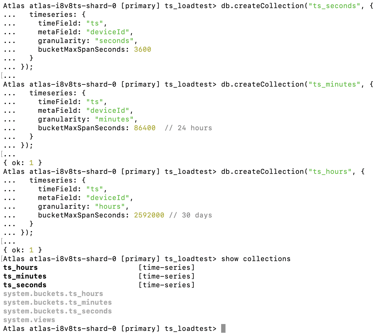
Before running any ingestion evaluations, all three time series collections, ts_seconds, ts_minutes, and ts_hours, were created empty and independently to ensure clean and isolated test conditions. Each collection uses the same timeField (ts) and metaField (deviceId), so measurements are consistently grouped by device across all scenarios. The only difference between the collections is the configured granularity, with bucketMaxSpanSeconds explicitly set to match MongoDB’s recommended defaults: one hour for seconds, twenty-four hours for minutes, and thirty days for hours. Creating these collections upfront ensures that observed differences in bucket behavior and query performance are driven solely by ingestion rate and granularity, rather than by residual data or implicit defaults.
Figure 1. Creation of collections (ts_seconds, ts_minutes, and ts_hours) with their granularity.
The PM2 process list shows all producers, consumers, and aggregation jobs used during the evaluations. Each component was run as an independent process to isolate ingestion, consumption, and analysis workloads. At the time of capture, all processes are intentionally stopped, confirming that no background ingestion or aggregation is influencing the results. This ensures that each run starts from a clean and controlled state.
Figure 2. Application environment to initiate load on time series collections and infrastructure.
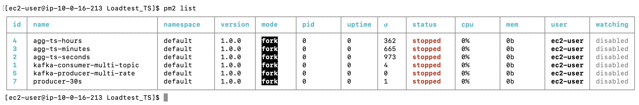
producer-30s – Generates time series data at a fixed 30-second interval and publishes it to Kafka topics.
kafka-producer-multi-rate – Publishes high-ingestion-rate time series messages to Kafka to simulate sustained write-heavy workloads.
kafka-consumer-multi-topic – Consumes time series messages from multiple Kafka topics and persists them into MongoDB time series collections.
agg-ts-seconds – Runs aggregation and benchmark queries on the ts_seconds collection to analyze bucket behavior and query performance.
agg-ts-minutes – Performs the same analysis on the ts_minutes collection configured with minute-level granularity.
agg-ts-hours – Executes aggregation and benchmarking logic on the ts_hours collection configured with hour-level granularity.
High ingestion rate (200 messages every 5 seconds)
In this evaluation, data is ingested at a high and uniform rate of 200 messages every 5 seconds into three time series collections: ts_seconds, ts_minutes, and ts_hours, each configured with seconds, minutes, and hours granularity, respectively. The expectation is that all three collections will receive data at the same rate, regardless of granularity, because the ingestion speed is high enough that buckets do not remain open long enough to close based on time. Instead, bucket rotation is driven primarily by internal size limits.
Under these conditions, MongoDB is expected to stop appending new measurements to a bucket once it reaches its internal size limits, approximately 1,000 measurements per bucket, and immediately begin writing to a new bucket, rather than continuing to reuse the existing one. Since the data is partitioned by the deviceId metaField (with 10 devices in this setup), each device maintains its own independent stream of buckets, and new buckets are created per device as earlier ones reach their lifecycle boundaries. Closed buckets are no longer involved in write operations and are treated like regular persisted data, becoming eligible for eviction from memory based on normal storage engine cache behavior. Granularity continues to define the maximum time span a bucket may cover, but at high ingestion rates, it is the size limit, not time, that determines when MongoDB transitions writes to a new bucket, allowing the system to sustain throughput while keeping memory and CPU usage stable across all three collections.
Infrastructure and collection details
Machine size: M30 (2vCPUs , 8 GB RAM)
Disk Size: 20 GB
Namespace 1: ts_loadtest.ts_seconds , Granularity : Seconds
Namespace 2: ts_loadtest.ts_minutes , Granularity : minutes
Namespace 3: ts_loadtest.ts_hours , Granularity : hour
Interpreting bucket behavior across granularities (observed output)
Across all three collections—ts_seconds, ts_minutes, and ts_hours—the benchmark output shows a consistent pattern: bucket creation and rotation are primarily driven by ingestion rate and metaField cardinality, not granularity alone. Each device (deviceId) maintains its own independent stream of buckets, which is why the “Buckets per Device” section consistently shows one or two buckets per device, depending on how long ingestion was allowed to run.
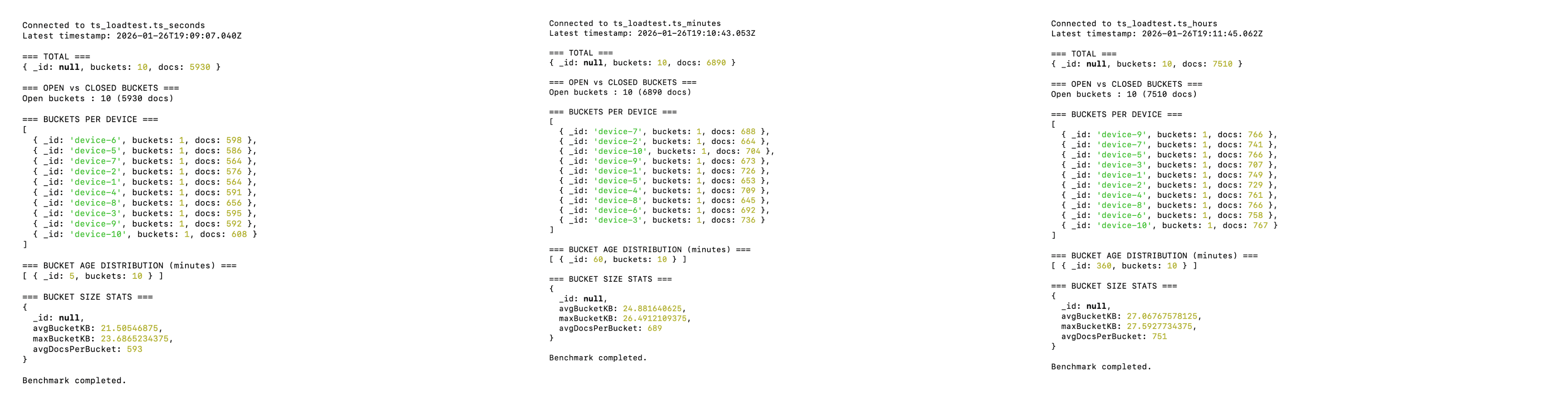
In this evaluation, ingestion was sustained for approximately 15 minutes. For the first 10 minutes, MongoDB did not create additional buckets because the active buckets had not yet reached the internal size threshold of roughly 1,000 measurements. During this period, MongoDB continued appending new measurements to the existing buckets, avoiding unnecessary bucket proliferation. Once the threshold was reached around the 15-minute mark, MongoDB transparently began writing to new buckets while leaving the previously filled buckets untouched. This transition happens without any application-level intervention and illustrates how MongoDB optimizes write locality and minimizes overhead under sustained ingestion.
In this high-ingestion scenario, granularity does not play a dominant role in bucket rotation, because size-based limits are reached well before any time-based span expires. Granularity instead defines the maximum duration a bucket is allowed to remain open. Once an untouched bucket reaches its configured time span, it becomes fully inactive and behaves like regular persisted data. At that point, memory residency is governed by the general WiredTiger cache eviction process, not by time series-specific logic, ensuring that backend memory usage remains stable and predictable.
Figure 3. First 10 Minutes of Test, only one bucket for each DeviceId as shown below.
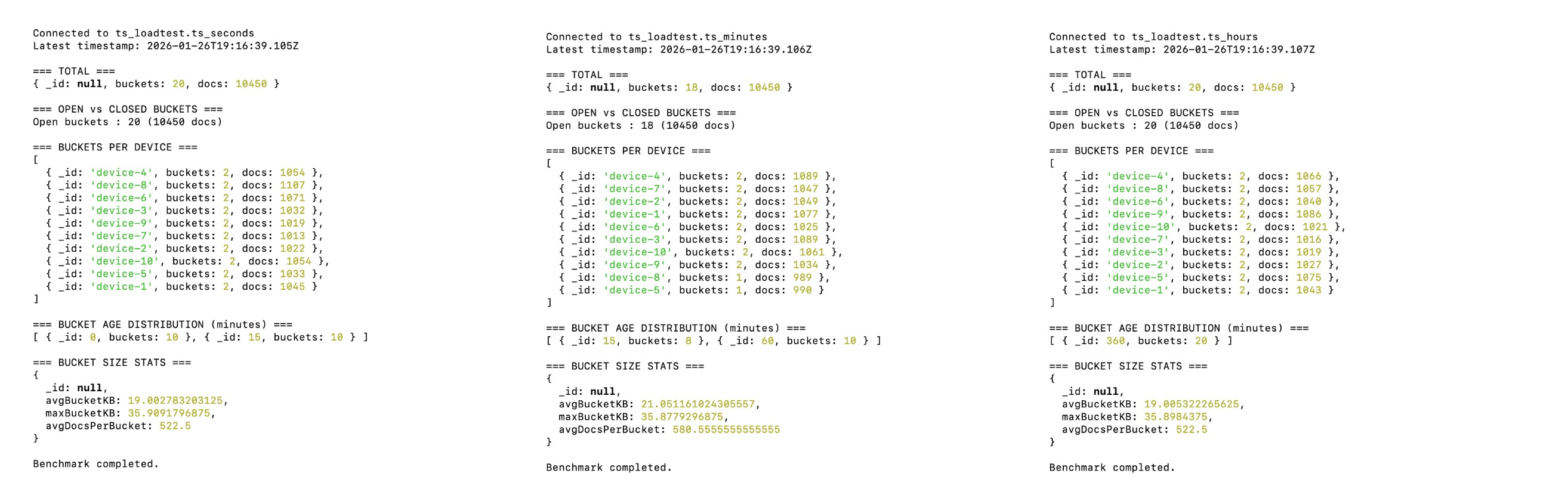
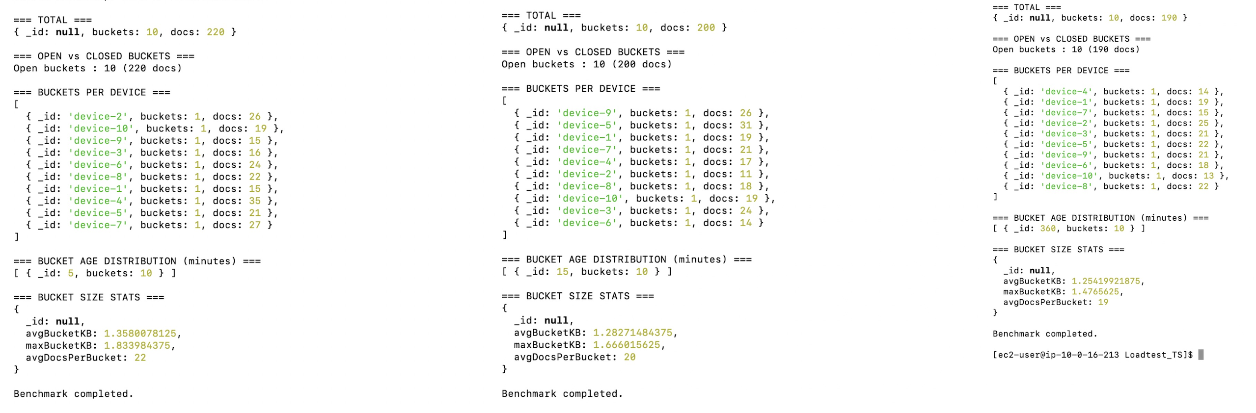
At around the 15-minute mark, all devices stop appending new measurements to their first active buckets and begin writing to new buckets. This behavior clearly demonstrates that, under high ingestion rates, bucket rotation in MongoDB time series collections is governed by the bucket’s upper limits rather than by the time span defined by granularity.
Figure 4. At the 15th minute, as the ingestion rate is high, all granularities created new buckets after 1000 measurements.
Low ingestion rate (10 messages every 30 seconds)
This low ingestion rate was chosen deliberately to demonstrate how time series bucket behavior changes when data arrives infrequently and how this pattern helps applications use memory more efficiently. MongoDB handles high ingestion rates well, as shown earlier. This scenario is presented to help users understand that by identifying an optimal ingestion window for their workload, they can make more effective use of infrastructure resources, achieving a better balance between cost efficiency and query performance.
The same infrastructure was used for the low ingestion rate evaluation. The results are presented below.
During the first 2 minutes of ingestion, all three time series collections—ts_seconds, ts_minutes, and ts_hours—maintain a single active bucket per device, with bucket sizes remaining well below the size thresholds. Since buckets do not reach the document or size limits, MongoDB continues appending to the same bucket and avoids creating new ones. In this scenario, granularity becomes the dominant factor, determining how long a bucket remains open before aging out, while memory usage stays efficient as inactive buckets are managed through the standard WiredTiger cache eviction process.
Figure 5. For the first 5 minutes, as the ingestion rate is low, all granularities are able to work with a single bucket.
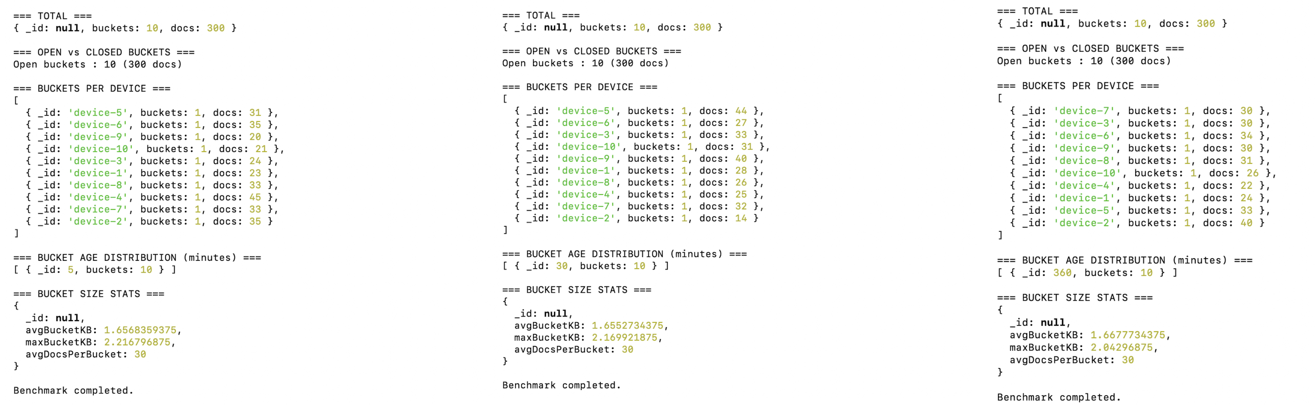
At the 5-minute mark, the low ingestion rate continues to produce the same fundamental behavior observed at 5 minutes: each device maintains a single active bucket, and bucket sizes remain well below the size thresholds. The key difference is visible in the bucket age distribution, where buckets now reflect longer lifespans aligned with their configured granularity (5 minutes for ts_seconds, 30 minutes for ts_minutes, and 360 minutes for ts_hours). This confirms that, under low ingestion, MongoDB does not create new buckets prematurely; instead, it allows existing buckets to age naturally, with granularity—not ingestion rate—governing bucket lifecycle.
Figure 6. At the 15th minute, as the ingestion rate is low now, the bucket behaviour is controlled by granularities.
Key Takeaway
This study demonstrates that MongoDB time series bucket behavior is governed by a combination of ingestion rate, granularity, and metaField cardinality, rather than granularity alone. Under high ingestion rates, buckets rotate quickly as size thresholds are reached, making granularity largely irrelevant to bucket creation. Under low ingestion rates, bucket rotation becomes time-driven, and granularity plays a critical role in determining bucket lifespan, query fan-out, and memory efficiency. By understanding how these factors interact, teams can make informed design choices that balance performance, cost, and operational stability. The key takeaway is to align ingestion patterns and granularity with real-world workloads, rather than optimizing for extremes, to fully leverage MongoDB’s time series architecture.
Next Steps
For more information, visit the MongoDB Time Series documentation.